![]()
Contenidos
Tema anterior
Clase 13: Ortogonalización de Gram-Schmidt
![]()
Clase 13: Ortogonalización de Gram-Schmidt
Bibliografía de la Clase
- Numerical Linear Algebra. L.N. Trefethen. Chapter 1: Lecture 10 Householder Triangularization
- Guía profesor Luis Salinas
Si se recuerda el algoritmo Gram-Schmidt Modificado , en forma matricial se tiene lo siguiente:
(i=1)
![\left[ \begin{array}{c|c|c|c}
\, & \, & \, & \, \\
\, & \, & \, & \, \\
v_1 & v_2 & \cdots & v_n \\
\, & \, & \, & \, \\
\, & \, & \, & \,
\end{array} \right]
\mathop{ \left[ \begin{array}{c|c|c|c|c}
1/r_{11} & -r_{12}/r_{11} &-r_{13}/r_{11} &\cdots & -r_{1n}/r_{11} \\
0 & 1 & 0 &\cdots & 0 \\
0 & 0 &1 & \cdots & 0 \\
\vdots & \vdots & \vdots & & \vdots\\
0 & 0 & 0 & \cdots & 1
\end{array} \right]}_{R_1}=
\left[ \begin{array}{c|c|c|c}
\, & \, & \, & \, \\
\, & \, & \, & \, \\
q_1 & v_2^{(1)} & \cdots & v_n^{(1)} \\
\, & \, & \, & \, \\
\, & \, & \, & \,
\end{array} \right]](_images/math/44f474f912891778a8c425d5728ec3394ec22859.png)
Para obtener  :
:
![\left[ \begin{array}{c}
\\
\\
q_1 \\
\\
\\
\end{array} \right]=
\left[ \begin{array}{c|c|c|c}
\, & \, & \, & \, \\
\, & \, & \, & \, \\
v_1 & v_2 & \cdots & v_n \\
\, & \, & \, & \, \\
\, & \, & \, & \,
\end{array} \right]
\left[ \begin{array}{c}
\\
\\
r_1 \\
\\
\\
\end{array} \right]=
v_1 \frac{1}{r_{11}}](_images/math/1091fac026a744f526cce999ab90608ad402f594.png)
Para obtener  :
:
![\left[ \begin{array}{c}
\\
\\
v_2^{(1)} \\
\\
\\
\end{array} \right]=
\left[ \begin{array}{c|c|c|c}
\, & \, & \, & \, \\
\, & \, & \, & \, \\
v_1 & v_2 & \cdots & v_n \\
\, & \, & \, & \, \\
\, & \, & \, & \,
\end{array} \right]
\left[ \begin{array}{c}
\\
\\
r_2 \\
\\
\\
\end{array} \right]=
v_1 -\frac{r_{12}}{r_{11}} + v_2 \ 1 + v_3 \ 0 + \ldots= v_2 - r_{12} q_1](_images/math/d9ad25119c1cd28a40199ac2778a9453e1f68938.png)
Para obtener  :
:
![\left[ \begin{array}{c}
\\
\\
v_3^{(1)} \\
\\
\\
\end{array} \right]=
\left[ \begin{array}{c|c|c|c}
\, & \, & \, & \, \\
\, & \, & \, & \, \\
v_1 & v_2 & \cdots & v_n \\
\, & \, & \, & \, \\
\, & \, & \, & \,
\end{array} \right]
\left[ \begin{array}{c}
\\
\\
r_3 \\
\\
\\
\end{array} \right]=
v_1 -\frac{r_{13}}{r_{11}} + v_2 \ 0 + v_3 \ 1 + \ldots= v_3 - r_{13} q_1
\ldots](_images/math/6d0ceff9f0453a0355b708f6f20d4a845c918e9f.png)
(i=2)
![\left[ \begin{array}{c|c|c|c}
\, & \, & \, & \, \\
\, & \, & \, & \, \\
q_1 & v_2^{(2)} & \cdots & v_n^{(2)} \\
\, & \, & \, & \, \\
\, & \, & \, & \,
\end{array} \right]
\left[ \begin{array}{c|c|c|c|c}
1 & 0 &0 &\cdots & 0 \\
0 & 1/r_{22} & -r_{23}/r_{22} &\cdots & -r_{2n}/r_{22} \\
0 & 0 &1 & \cdots & 0 \\
\vdots & \vdots & \vdots & & \vdots\\
0 & 0 & 0 & \cdots & 1
\end{array} \right]=
\left[ \begin{array}{c|c|c|c}
\, & \, & \, & \, \\
\, & \, & \, & \, \\
q_1 & q_2 & \cdots & v_n^{(2)} \\
\, & \, & \, & \, \\
\, & \, & \, & \,
\end{array} \right]](_images/math/837376e4f60c6ac1521683f9627da5eed585ff65.png)
Para obtener  :
:
![\left[ \begin{array}{c}
\\
\\
q_2 \\
\\
\\
\end{array} \right]=
\left[ \begin{array}{c|c|c|c}
\, & \, & \, & \, \\
\, & \, & \, & \, \\
v_1 & v_2 & \cdots & v_n \\
\, & \, & \, & \, \\
\, & \, & \, & \,
\end{array} \right]
\left[ \begin{array}{c}
\\
\\
r_1 \\
\\
\\
\end{array} \right]=
v_2 \frac{1}{r_{22}}](_images/math/25a6d2d8fa7d68282d634f1d90d723c93b34db90.png)
Para obtener  :
:
![\left[ \begin{array}{c}
\\
\\
v_3^{(2)} \\
\\
\\
\end{array} \right]=
\left[ \begin{array}{c|c|c|c}
\, & \, & \, & \, \\
\, & \, & \, & \, \\
v_1 & v_2 & \cdots & v_n \\
\, & \, & \, & \, \\
\, & \, & \, & \,
\end{array} \right]
\left[ \begin{array}{c}
\\
\\
r_2 \\
\\
\\
\end{array} \right]=
v_2^{(1)} -\frac{r_{23}}{r_{22}} + v_3^{(1)}
\ldots](_images/math/77427708b6f2bbcd78faca346fed4b70b30bb033.png)
Idea
Mediante las iteraciones del método de Gram-Schmidt se aplica una
sucesión de matrices triangulares superiores  por la derecha de la
matriz
por la derecha de la
matriz  (aunque en la práctica no formamos las matrices
  ):
):
y la matriz resultante,  tiene columnas ortonormales. El producto
 es una matriz triangular superior,
obteniendo así la factorización QR reducida de A.
es una matriz triangular superior,
obteniendo así la factorización QR reducida de A.
Por otro lado, el método de Householder aplica una sucesión de matrices
unitarias  por la izquierda de A:
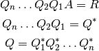
y la matriz resultante  , es una matriz triangular superior. El producto
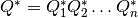 es también una matriz unitaria,
por lo que se obtiene la factorización QR completa de .
es también una matriz unitaria,
por lo que se obtiene la factorización QR completa de .
Resumen:
Por lo tanto, ambos métodos pueden resumirse de la sgte. manera:
Gram-Schmidt: Ortogonalización triangular
Householder: Triangularización ortogonal.
Este método fue propuesto por Alston Householder en el año 1958, y es una forma
ingeniosa de diseñar matrices unitarias , que realicen las siguientes operaciones:
![\mathop{\left[ \begin{array}{c c c}
x &x & x \\
x &x & x \\
x &x & x \\
x &x & x \\
x &x & x \\
\end{array} \right]}_{A} \mathop{\longrightarrow}^{Q_1}
\mathop{\left[ \begin{array}{c c c}
* &* & * \\
0 &* & * \\
0 &* & * \\
0 &* & * \\
0 &* & * \\
\end{array} \right]}_{Q_1 A} \mathop{\longrightarrow}^{Q_2}
\mathop{ \left[ \begin{array}{c c c}
x &x & x \\
0 &* & * \\
0 &0 & * \\
0 &0 & * \\
0 &0 & * \\
\end{array} \right]}_{Q_2 Q_1 A} \mathop{\longrightarrow}^{Q_3}
\mathop{\left[ \begin{array}{c c c}
x &x & x \\
0 &x & x \\
0 &0 & * \\
0 &0 & 0 \\
0 &0 & 0 \\
\end{array} \right]}_{Q_3 Q_2 Q_1 A}](_images/math/eb62566611f4d366431ff82200a4b12763b4829a.png)
 elemento de la matriz, no necesariamente cero.
 elemento que se ha modificado recientemente.
En general, opera sobre las filas  .
.
La matriz tiene la siguiente forma:
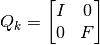
 es la matriz identidad y tiene dimensión
 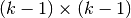 .
.
 es el Reflector de Householder y tiene dimensión
  , y es una matriz unitaria.
tiene dimensión 
En la iteraciónse transforma el vector
. El reflector de Householder realiza la siguiente transformación:
Reflexión de Householder:
 va a reflejar el espacio
  (o
(o  , más fácil de “visualizar”) a través del hiperplano
  que es ortogonal a
  .
. , corresponde a este vector.
La fórmula de la reflexión se puede derivar de la siguiente forma:
¡Pero es necesario reflejar! Por lo tanto se debe detener en el punto anterior, sino que avanzar dos veces en la misma dirección:
Ejercicio en Clases
Demostrar, geométricamente, que el reflector de Householder es  .
.
 sobre ? sobre ? sobre ?
Existen varios reflectores de Householder:  como
como  .
.

El vector puede ser reflejado a  , donde
  es escalar con
  . Si
. Si
 circunferencia con posibles reflexiones, si
  2 posibles reflexiones, correspondientes al hiperplano
  y
y  .
.
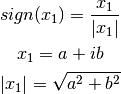
Matemáticamente, ambas transformaciones son correctas, pero para un dado,
se busca estabilidad numérica, para lo cual se escoge la reflexión más
lejana a .
Para lograr esto se escoge:
Recordar:
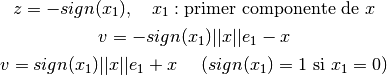
Si  :
:
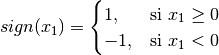
Recordar:
Si  :
:


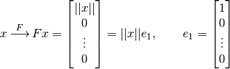
Ejemplo
Iteración 1:
.
![\mathop{\left[ \begin{array}{c c c}
x_1 &* &* \\
x_2 &* &* \\
x_3 &* &* \\
x_4 &* &* \\
x_5 &* &* \\
\end{array} \right]}_{A}
\rightarrow x = \begin{bmatrix} x_1 \\ x_2 \\ x_3 \\ x_4 \\ x_5 \end{bmatrix} \in \mathbb{C}^{5}, \ \ \ e_1 = \begin{bmatrix} 1 \\ 0 \\ 0 \\ 0 \\ 0 \end{bmatrix} \in \mathbb{C}^{5}
v_1=sing(x_1) ||x|| e_1 + x
\vspace{0.5cm}
P=\frac{v_1 v_1^*}{v_1^* v}
\vspace{0.5cm}
\text{dim}(I) = (k-1) \times (k-1) = 0 \times 0
\text{dim}(F) = (m-k+1) \times (m-k+1) = 5 \times 5
\vspace{1cm}
Q_1= F_1= \left[ \begin{array}{c c c c c}
F &F &F &F &F \\
F &F &F &F &F \\
F &F &F &F &F \\
F &F &F &F &F \\
F &F &F &F &F \\
\end{array} \right]_{5\times 5} = I-2\frac{v_1 v_1^*}{v_1^* v}](_images/math/d307c91745d451b97a3374c5815e1d4299b7f55b.png)
Iteración 2:
.
![\mathop{\left[ \begin{array}{c c c}
R &R &R \\
0 &x_1 &* \\
0 &x_2 &* \\
0 &x_3 &* \\
0 &x_4 &* \\
\end{array} \right]}_{A}
\rightarrow x = \begin{bmatrix} x_1 \\ x_2 \\ x_3 \\ x_4 \end{bmatrix} \in \mathbb{C}^{4}, \ \ \ e_1 = \begin{bmatrix} 1 \\ 0 \\ 0 \\ 0 \end{bmatrix} \in \mathbb{C}^{4}
v_2=sing(x_1) ||x|| e_1 + x
\vspace{0.5cm}
P=\frac{v_2 v_2^*}{v_2^* v_2}
\vspace{0.5cm}
\text{dim}(I) = (k-1) \times (k-1) = 1 \times 1
\text{dim}(F) = (m-k+1) \times (m-k+1) = 4 \times 4
\vspace{1cm}
Q_2= F_2= \left[ \begin{array}{c c c c c}
1 &0 &0 &0 &0 \\
0 &F &F &F &F \\
0 &F &F &F &F \\
0 &F &F &F &F \\
0 &F &F &F &F \\
\end{array} \right]_{5\times 5} = I-2\frac{v_2 v_2^*}{v_2^* v_2}](_images/math/ae72084015a5057b5225e53615771abcffcba9e6.png)
Iteración 3:
.
![\mathop{\left[ \begin{array}{c c c}
R &R &R \\
0 &R &R \\
0 &0 &x_1 \\
0 &0 &x_2 \\
0 &0 &x_3 \\
\end{array} \right]}_{A}
\rightarrow x = \begin{bmatrix} x_1 \\ x_2 \\ x_3 \end{bmatrix} \in \mathbb{C}^{3}, \ \ \ e_1 = \begin{bmatrix} 1 \\ 0 \\ 0 \end{bmatrix} \in \mathbb{C}^{3}
v_3=sing(x_1) ||x|| e_1 + x
\vspace{0.5cm}
P=\frac{v_3 v_3^*}{v_3^* v_3}
\vspace{0.5cm}
\text{dim}(I) = (k-1) \times (k-1) = 2 \times 2
\text{dim}(F) = (m-k+1) \times (m-k+1) = 3 \times 3
\vspace{1cm}
Q_3= F_3= \left[ \begin{array}{c c c c c}
1 &0 &0 &0 &0 \\
0 &1 &0 &0 &0 \\
0 &0 &F &F &F \\
0 &0 &F &F &F \\
0 &0 &F &F &F \\
\end{array} \right]_{5\times 5} = I-2\frac{v_3 v_3^*}{v_3^* v_3}
\Rightarrow \left[ \begin{array}{c c c}
R &R &R \\
0 &R &R \\
0 &0 &R \\
0 &0 &0 \\
0 &0 &0 \\
\end{array} \right]](_images/math/6c195b4f097019a5374ba041a4d23efc667abca7.png)
Ejercicio:
, utilizando la triangularización de Houselder: