Bibliografía de la Clase
- Numerical Linear Algebra. L.N. Trefethen. Chapter 2, Lecture 11: Least Squares Problems
- Guía profesor Luis Salinas
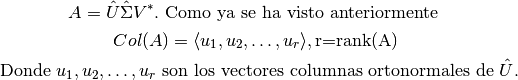
 y
y 
 es la proyección ortogonal de
  sobre
sobre  , i.e.,
  , donde
  para algún
  , por lo tanto .

y  :
:

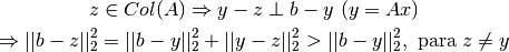

Además,
Por otro lado,
Por lo tanto,
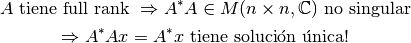
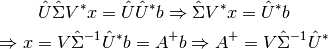
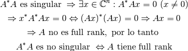
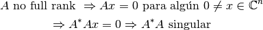
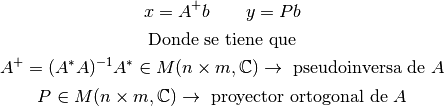
Si  es full rank, la solución de
  está dada por:
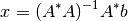
 se denomina la pseudoinversa de , y se denota
  . transforma el vector al vector , lo que explica que tiene dimensión
  (más columnas que filas).
Resumiendo:
El problema de mínimos cuadrados consiste en calcular alguno de los sgtes. vectores:
¿Cómo calcular los vectores e  ?
?
Utilizando las ecuaciones normales:

 puede ser de la forma:
  , que permite obtener la proyección de
  sobre .
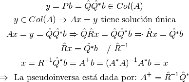
Ventajas